Accounting

No matter what company it is, the maintenance of correct financial records is crucial in determining its financial performance. At the end of each month, the month-end closing process takes place, which helps in recording financial transactions, reconciling financial accounts, and providing financial data. The process of month-end closing is not just about verifying numbers at the end of the month. In fact, the process of month-end closing consists of reviewing transactions, reconciling accounts, making adjustments, detecting errors and preparing financial statements. This process of month-end closing helps companies maintain correct books and helps management know their financial performance.

Understanding the Financial Closing Process

The financial closing process is a systematic procedure used by accounting teams to finalise financial records for a specific accounting period. While the exact activities may vary depending on the size and nature of an organisation, the objective remains the same: to make sure that the financial data for the month is complete, accurate, and properly documented.

The accountant gathers data from various departments, verifies the transaction details, reconciles accounts, makes journal entries, and checks the financial statements during the closing process. Many companies rely on accounting software and ERP systems for their closing activities.

Reviewing and Recording Financial Transactions

The initial step in month-end closing is to check that all the financial transactions for the month have been recorded properly. The accountants will analyse sales invoices, purchase invoices, receipts, payments, payroll transactions, expense invoices, and other related transactions.

If there are any transactions that have not been recorded or those which have been recorded incorrectly, it could greatly impact the preparation of the financial statements. Thus, the accounting staff members reconcile the transactions with the documentation, if necessary.

Reconciling Bank and Other Accounts

Account Reconciliation is an essential component of the closing process. Accountants reconcile the books of a business with outside documents, such as the bank statement, credit card statement, among others.

The bank reconciliation can help uncover discrepancies due to outstanding cheques, bank service charges, deposits in transit, errors, or transactions that have not been recorded in the accounting system. This will ensure the accuracy of the accounting information.

Managing Accounts Receivable and Payable

The closing process also requires a detailed review of accounts receivable and accounts payable. The accounting team checks whether customer invoices have been recorded correctly and whether outstanding receivables are properly reflected in the books.

At the same time, accountants review supplier invoices, pending payments, and unpaid expenses. This provides a clearer understanding of the company’s short-term obligations and expected cash inflows. Regular monitoring of receivables and payables can also help organisations improve cash-flow management.

Recording Adjusting Entries

It should also be noted that not all financial transactions are automatically recorded through routine transactions. Some incomes and expenditures have to be accounted for through adjustments at the end of an accounting period.

Such incomes and expenditures may include depreciation, accruals, prepayments, provisions, or accrued incomes. Adjustments allow for the recording of incomes and expenditures in accordance with generally accepted accounting practices.

Checking Payroll and Employee Expenses

Other areas include Payroll, which also needs focus in the month-end closing process. Accounting personnel review salaries, allowances, rebates, bonuses, perks and other personnel-related expenses.

Any outstanding personnel expense or liability related to payroll needs to be accrued prior to finalising the accounts. Proper Payroll accounting helps ensure proper allocation of personnel expenses within the appropriate reporting period.

Reviewing General Ledger Accounts

When postings have been done and adjustments have been made, the accounts in the general ledger are analysed for irregularities, duplicated entries, misclassifications, or other irregularities. It is especially critical to perform this analysis since mistakes in any particular account might impact many different parts of the accounting records of the business. Accountants might compare the amounts in the current month to previous periods or budgets.

Preparing Financial Reports

Once the accounts have been analysed and adjusted, the financial department can start preparing financial statements. Financial statements can be divided into the income statement, balance sheet, cash flow statement, trial balance, and management accounting statements.

Accurate financial reporting enables business leaders to understand revenue trends, operating costs, profitability, liquidity, and financial obligations. These reports also support budgeting, forecasting, strategic planning, and decision-making.

Reviewing and Approving the Final Numbers

The process of closing the accounting period starts with senior accountants or finance managers reviewing the final numbers. Account balances, adjustments, reconciliations, and financial statements are checked for reasonableness and proper support. When any discrepancies are found, they are investigated and corrected prior to final approval.

This adds another level of quality control, decreasing the chances of wrong information getting to the management or other stakeholders.

Closing the Accounting Period

After completing all the reviews and necessary corrections, the accounting period is now closed. After closing the period, companies can impose some restrictions on the further posting of entries to avoid any changes made to the finalised data.

The prepared documents serve as a basis for the preparation of the report, audits, tax work, budgeting, and the accounting period ahead. Proper documentation of all the procedures also simplifies future reviews and audits.

Why an Efficient Financial Closing Process Matters

A well-organised financial closing process helps organisations produce accurate financial information within a predictable timeframe. When closing activities are delayed or performed without proper controls, businesses may experience reporting errors, compliance problems, inaccurate forecasts, and poor financial decisions.

While modern accountants have been using ERP systems, accounting software, automation and standardisation of the closing process to increase efficiency, it cannot be achieved without accounting expertise. The knowledge of accounting principles, reconciliations, journal entries, financial statements, and the reporting process is required for accountants to recognise issues and make decisions.

Building a Career in Accounting and Finance

Learning about the month-end processes may be important for students and specialists who want to build their careers in the field of accounting, finance, or business operations. Acquiring practical skills in the areas of bookkeeping, tax accounting, financial statements, ERPs, and accounting software may be helpful for learners.

For individuals looking to develop practical industry skills, Job-Oriented courses in Bangalore can provide structured learning combined with hands-on exposure. Choosing training that focuses on real accounting scenarios, software applications, and workplace processes can help learners bridge the gap between academic knowledge and professional requirements.

Conclusion

The month-end closing process is a crucial step in accounting that entails several processes such as recording transactions, reconciling accounts, making adjustments, analysing ledgers, and preparing the financial statements. The main aim of this process, despite having many steps of verification, may not be as complex as it looks.

A consistent month-end closing process will enable firms to get good financial information and hence make sound business decisions. Aspiring accounting professionals will benefit greatly from learning the month-end closing process.

Frequently Asked Questions

1. What is the month-end closing process?

It is the process of checking, matching, and closing a company’s accounts at the end of each month

2. How long does month-end closing last?

The duration varies from a few days up to one week or even longer, based on the complexity of a business.

3. What is included in the financial closing process?

This process includes reviews, account reconciliations, adjustment journal entries, and preparing financial statements.

4. Why is the month-end closing process important?

The month-end closing process helps to ensure the accuracy of accounting records.

5. Can accounting software aid in month-end closing?

Accounting software can be very helpful in this regard.

Generally, buying a laptop, a vehicle, machinery, office equipment, and buildings by organisations is not merely an act, but it goes much further because these are essential in facilitating the operations of the business. But from an accounting perspective, buying a property is only one part of the entire process. It has to be identified, recognised, valued, depreciated, maintained, and finally disposed of once the asset has been sold or is no longer useful.

Thus, it is important to know the entire process in order to avoid mistakes at each stage since they may cause problems in the financial statements, the level of profitability, and taxation, among others. That is why fixed assets in accounting must be understood beyond buying.

What Are Fixed Assets in Accounting?

Fixed assets refer to physical assets that are owned by a company for use in its activities and are expected to be held for more than one accounting period. Examples of fixed assets include buildings, machinery, vehicles, computers, furniture, office equipment, among others. As per IAS 16, property, plant and equipment is only recognised as an asset if there are future economic benefits that are probable and the cost of the asset can be measured reliably.

While most costs incurred by a company are expensed immediately as per IAS 37 – Provisions, Contingent Liabilities, Contingent Assets, a fixed asset is different in that it confers economic benefits over a longer period. When a company acquires a computer for use by its finance department, the entire cost of the computer would not normally be expensed.

The First Stage: Identifying and Planning the Asset Purchase

The life cycle starts even before the arrival of the asset at the premises of the company. The company will first realise that there is a need for the particular asset and that its purchase will be economically or operationally profitable. There are various considerations such as supplier evaluation, price comparison, specifications, financial evaluation of the life of the asset, maintenance cost, and others before the decision to purchase the asset is made by the management.

From the accounting point of view, this is very crucial in ensuring that the accounting department is provided with enough documentation regarding the asset and the cost incurred for its procurement.

Acquisition and Initial Recognition

After the purchase of the asset, the accounting department will decide whether the asset needs to be capitalised or treated as expenses based on the existing accounting policies and criteria of the organisation.

The initial cost of qualifying property, plant, and equipment according to IAS 16 comprises the purchase price and all additional costs required to get the asset ready for use in the conditionin whiche it is intended to be used. Some estimates of dismantling, removal, and restoration costs can also be included in the initial cost of the asset.

For instance, if an organisation acquires manufacturing equipment, the accounting department may take into account the purchase price, delivery costs, setup costs, and any other relevant costs while calculating the initial carrying amount of the asset. The idea is to make sure that the asset is correctly valued initially and not merely recorded using the figure from the vendor’s invoice.

Recording the Asset in the Fixed Asset Register

Following recognition, the asset should be entered into the organisation’s fixed asset register. The fixed asset register is used by the finance team to keep an account of the organisation’s assets.

Information that may be recorded in the asset register may include the description of the asset, the asset code number, date of purchase, vendor, original cost, location, department in charge, useful life, method of depreciation, total depreciation and book value. It becomes very crucial for a business organisation that has numerous assets to maintain accurate records of those assets.

An accurate asset register facilitates comparisons between accounting records and actual assets on the ground. For example, the organisation may have accounted for a computer but is unable to identify the actual computer.

Determining Useful Life and Residual Value

Once an asset is recognised, there comes the need to find out the period that the asset is expected to provide benefits and its possible residual value at the end of the period. Useful life does not always coincide with the maximum physical life of the asset. Useful life is defined in terms of the period of time during which the asset is expected to be used within the business or the number of production or similar units from the asset.

For instance, while a company might have the expectation that a laptop could still be in good condition after some years, it is replaced early due to technological changes and other reasons. Useful-life estimates are affected by such factors as expected usage, maintenance, technological changes, and legal and contractual constraints.

Residual value is important since the estimation of depreciation is done on the basis of the depreciable amount, which takes into account the residual value of the asset. Useful life and residual value estimates should not just be taken as fixed. IAS 16 requires the useful life and residual value to be reviewed annually.

Depreciation: Allocating the Asset’s Cost

Depreciation is among the key phases within the life cycle of an asset. Rather than expensing all the cost of acquisition of a depreciating asset, the cost is expensed gradually over the period of the useful life of the asset.

This impacts the income statement and balance sheet, where depreciation expense is recorded against accumulated depreciation that lowers the value of the asset. One may consider preparing a depreciation schedule in order to assist the finance team in keeping track of the original cost of assets, depreciation expense, accumulated depreciation, and book value.

The depreciation rate must correspond to the expected way in which economic benefits from the asset will be used up. In accordance with IAS 16, businesses may use various methods such as straight-line depreciation, etc. It is necessary to remember that IAS 16 suggests that depreciation starts when an asset is available for use, which means that it is ready to function in its intended place and condition.

Thus, precise calculation of depreciation is crucial. The wrong start date, useful life, residual value, or method leads to incorrect reporting.

Monitoring, Maintenance, and Subsequent Costs

An asset’s life cycle is not a passive process once depreciation has commenced. A business needs to keep track of its assets during the period when they are being used in operations. Assets such as machinery may need repair work, upgrading, replacement, inspection, or enhancement.

The accounting staff must determine whether the cost incurred is one that requires the recognition of the expenditure within the carrying amount of the asset or if the cost is one that needs to be charged against the current income.

Monitoring assists companies in determining any damage, obsolescence, idleness, or poor performance of assets.

Physical Verification and Reconciliation

As organisations expand, discrepancies may arise between the fixed asset ledger and the physical asset inventory. Assets could be shifted to another department, relocated to other branches, replaced, lost, or inaccurately accounted for.

Physical inspection assists businesses in ensuring that the assets listed in the accounting system indeed exist and are being used or controlled by the organisation. The finance department can reconcile asset ID numbers, locations, descriptions, and condition against the fixed asset ledger.

This is particularly useful during audits since there will be stronger evidence that the asset balances maintained by the organisation are accurate.

Impairment and Changes in Asset Value

At times, the decline in value may occur much faster than what was originally anticipated. The decline in value may be due to damage, obsolescence of technology, market conditions, and economic benefits, among others.

The difference between impairment and depreciation is that, whereas depreciation is an allocation process, impairment arises in cases where the carrying amount might no longer be recoverable. The Impairment of Assets Standard, IAS 36, provides the accounting treatment of property, plant, and equipment, which is the same as that covered in IAS 16.

Transfer, Retirement, and Disposal

Ultimately, each asset comes to a point when the business decides to dispose of it by either replacing it, selling it, or retiring it. This marks the final stage of the accounting life cycle of an asset.

Prior to disposal, the accountant must calculate the carrying amount of the asset based on the cost of the asset and its accumulated depreciation, plus other factors, if any. The asset and the related accumulated depreciation are then written off from the accounting records as needed.

Where there is a sale of the asset at an amount that is not equal to its carrying amount, a profit or loss arises that will affect the income statement. Asset disposal thus calls for proper recording and proper accounting treatment.

For instance, consider a machine that is initially recorded at ₹10 lakh while its accumulated depreciation is ₹7 lakh, giving it a carrying amount of ₹3 lakh. In the event that the company sells the machine at ₹3.5 lakh, it will usually result in a ₹50,000 gain.

Final Reconciliation and Reporting

After disposal or retirement of a fixed asset, there is a need to ensure that the fixed asset register, general ledger, depreciation schedule, and any supporting documents are revised to avoid the situation where the disposed-of fixed asset stays active in the accounting records.

Under IFRS, IAS 16 mandates disclosure of all property, plant and equipment as per their classes, which include measurement bases, methods of depreciation, useful life or rate of depreciation, gross carrying amount, total depreciation, and movement in carrying amount.

From the above information, it is evident that fixed asset accounting is not just about acquisition.

Why Fixed Assets in Accounting Matter for Accounting Professionals

Knowledge about the accounting life cycle will enable accounting practitioners to confidently work with various business transactions since it will enable them to know how a transaction impacts the balance sheet, how depreciation impacts the bottom line, and how asset transfers and dispositions impact the financial statements.

The accounting and finance training will provide knowledge about concepts like journalizing transactions, depreciation, financial statement preparation, accounting reconciliation, taxation, and the use of accounting software. Practical learning is important because actual accounting involves not just learning definitions but also why transactions are made the way they are recorded and how they affect the financial position of an organisation as a whole.

Those interested in structured learning will also be able to access one of the best accounting courses in Bangalore, where they learn accounting concepts along with practical tools and business situations. The hands-on training will make it easy for the learner to know how accounting transactions move from source documents to accounting software to financial statements.

Conclusion

The lifecycle of an asset involves identifying a business need followed by acquisition, recording, maintenance of the asset register, depreciation, monitoring, validation, assessing impairment, and finally disposing of the asset. Every one of these stages has its accounting implications and significance for financial statement preparation.

To the accountant, this whole concept of the fixed asset lifecycle is quite important since it is possible that fixed assets constitute a large part of the business’s resources. By having proper record-keeping, organisations will have an idea of their resources available to them, their performance, the value of these assets left, and whether or not they require replacing or disposing of.

Simply put, fixed asset management is all about managing an asset right from when it becomes part of the business organisation until when it is no longer required in the business.

Frequently Asked Questions’

What is the life cycle of fixed assets?

The life cycle normally encompasses planning and procurement, identification, accounting, depreciation, management, verification, valuation for possible impairment, and finally disposal or retirement.

Why is depreciation an important part of fixed asset accounting?

Depreciation involves the systematic allocation of the depreciable amount of an asset over its useful life and assists in the measurement of the consumption of economic benefits.

What is a fixed asset register?

A fixed asset register is a register that records details of assets, including details like date acquired, cost, location, useful life, depreciation, and carrying amount of assets.

When is a fixed asset retired?

Generally, an asset is retired once it is disposed of or when there will be no further economic benefit expected either from using or disposing of the asset.

Can accounting training assist in understanding fixed assets?

Absolutely yes. Accounting training can assist people in understanding asset identification, depreciation, reconciliation, journal entries, financial reporting, and accounting systems, among other concepts.

All businesses make investments in assets, which will generate income for them. Machines are needed to run the production plants; computers are needed for office work; delivery trucks are necessary to deliver the goods; and office furniture helps in creating productive offices. All of these are purchased by businesses at some cost, but the value of these assets decreases slowly due to various reasons.

Understanding depreciation methods is one of the most important accounting skills for students, finance professionals, and business owners. It is not just an accounting adjustment recorded at the end of the financial year. Instead, depreciation directly affects financial statements, taxation, profitability, budgeting, and business decision-making. Choosing the right method ensures that financial reports present a true and fair view of an organisation’s financial position.

Depreciation may appear to be difficult for a novice in accounting due to the various methods available to suit different circumstances. Fortunately, however, once the real-life purpose of each method is understood, choosing the right method is no longer difficult. The following is an explanation of various depreciation methods with the help of examples from real business life.

What Is Depreciation?

Depreciation is an allocation of the cost of the asset throughout its useful life. Rather than recognising the total cost of the asset all at once, firms recognise the expense in different accounting periods because the asset continues to generate income for the company during those accounting periods.

For instance, if a firm buys manufacturing equipment at a cost of $100,000 and the useful life of the asset is ten years, recognition of the total cost during the first year would distort the earnings of the company. Therefore, accounting standards prescribe that the firms recognise the total expense throughout the life of the asset.

Assets that are subject to depreciation include tangible assets like equipment, vehicles, office supplies, computers, furniture, and buildings. In general, land is exempt from depreciation since its value is not expected to depreciate over time.Knowledge of depreciation is important in learning about accounting principles since it incorporates the principle of matching, where the expenses are recognised during the same period as the revenues.

Why Choosing the Right Depreciation Method Matters?

Depreciation calculation should be done in accordance with the appropriate method, not only for compliance reasons. Some assets depreciate much faster in the early years, whereas others remain stable through the entire period of their use.

The selection of the right depreciation technique makes it easier for companies to:

• Present accurate financial statements
• Estimate asset replacement costs
• Calculate taxable income appropriately
• Improve budgeting and financial planning
• Measure departmental profitability more effectively
• Make informed investment decisions

Incorrect depreciation can lead to misleading financial reports, affecting lenders, investors, auditors, and management decisions.

Straight-Line Method

The Straight-Line Method is the simplest and most popular method. With this method, the same amount of depreciation is charged each year during the useful life of the asset.

The computation is simple:

(Asset Cost – Residual Value) ÷ Useful Life

Real Business Scenario

Think about a digital marketing agency buying office furniture at a cost of $30,000. This office furniture is supposed to serve for ten years, and the residual value will be $5,000.

The depreciation for each year will be:

($30,000 – $5,000) / 10 = $2,500

The company recognises a depreciation expense of $2,500 every year until the office furniture depreciates to its residual value.

This technique works best when applied to office furniture, buildings, classroom tools, and any asset that yields equal utility over its useful life.

Most educational bodies, consultancy firms, and service companies use this technique since it provides constant annual expenses.

Written Down Value Method

It is also referred to as the Declining Balance Method because it determines the depreciation amount using the residual book value of the asset rather than its original cost.

Thus, high depreciation amounts are incurred in the early years while the figures decline in subsequent periods.

Real Business Scenario

An information technology company buys servers for the price of $80,000.

Technology develops very fast, and thus the servers will depreciate very fast during the initial few years because of new products on the market.

The company does not use equal depreciation annually but rather uses the Written Down Value Method.

Assuming that the rate of depreciation is 25%.

Depreciation in Year One:

25% of $80,000 = $20,000

Remaining value: $60,000

Depreciation in Year Two:

25% of $60,000 = $15,000

Remaining value: $45,000

And so forth until the end of the asset’s useful life.

This depreciation method is preferred by companies with technology-based assets.

Units of Production Method

Certain assets are depreciated not according to time but usage. In such instances, the Units of Production Method provides a more realistic view of asset utilisation.

Depreciation will be calculated according to production levels and not according to years.

Real Business Scenario

A packing firm buys a machine that can produce one million units of carton throughout its useful life.

The cost of the machine is $120,000, while the scrap value is estimated to be $20,000.

Depreciation on a per-unit basis will be:

($120,000 – $20,000) ÷ 1,000,000 = $0.10 per carton

Now, if the machine manufactures 150,000 cartons in a year, depreciation will be:

150,000 x $0.10 = $15,000

And if in the following year more units are manufactured, depreciation will increase.

This approach is often used

Sum-of-the-Years’-Digits Method

With this approach to rapid depreciation, greater expenses are recognised at the beginning stages and decrease as time goes on.

Even though it is not very popular, it can be quite helpful in certain situations.

Real Business Scenario

The design studio buys special graphic workstations that are expected to be efficient for five years.

The firm expects the period when it will have maximum efficiency to be within the first few years until new technology comes on the market.

The Sum-of-the-Years’-Digits technique will enable the firm to depreciate more while the asset is still economically useful.

This is the matching principle of accounting.

Double Declining Balance Method

This method is another accelerated depreciation approach. It applies twice the straight-line depreciation rate to the asset’s current book value.

Businesses using expensive technological equipment often adopt this approach.

Real Business Scenario

There is a firm that uses modern machines that help in AI computation.

As the technology changes very rapidly, the firm selects the Double Declining Balance depreciation method.

Depreciation becomes higher in the early years as the machine loses its value faster and becomes inefficient.

It gives a practical view and helps in planning replacement.

Comparing the Different Methods

Different methods have varying business uses.

The Straight Line Method is used because it offers easy calculations and regular annual costs; thus, it is applicable for office property and buildings.

Written Down Value Method captures the fact that there is accelerated depreciation in the first few years, therefore useful in the depreciation of cars, computers and electronics.

Units of Production Method takes into account the depreciation that is dependent on the number of units of product produced, hence useful for industries whose production varies.

The Sum of Years Digits Method involves accelerated depreciation but follows a systematic process, while the Double Declining Balance Method is used in cases where the depreciation is highest in the initial period.

Choosing the best method should be based on the contribution of the asset to the business.

The Role of Depreciation in Financial Reporting

Depreciation influences almost every major financial report.

In the income statement, it appears as an operating expense, reducing the reported profit for the accounting period.

On the balance sheet, accumulated depreciation reduces the carrying value of fixed assets, allowing stakeholders to understand their remaining book value.

It also affects cash flow analysis indirectly. Although depreciation is a non-cash expense, it reduces taxable income, often improving operating cash flow.

This relationship is especially important in fixed asset accounting, where businesses must accurately track acquisition costs, accumulated depreciation, asset disposals, and remaining book values throughout an asset’s lifecycle.

Modern accounting software simplifies these calculations, but professionals still need a strong understanding of the underlying principles to verify reports and identify potential errors

Common Mistakes Businesses Make

Most businesses have problems associated with depreciation due to ignorance about the practical issues involved in asset management.

One such problem is overestimation or underestimation of the useful life of the asset. Overestimation results in underestimation of depreciation charges per year, while underestimation results in overestimation of depreciation charges per year.

Another common problem is that businesses do not revise their depreciation charges in case of changes in usage of the asset, for instance, due to any improvements.

Still another problem is the use of one method of calculating depreciation regardless of the type of asset, whether it be office furniture, manufacturing machinery, cars or computers.

Errors in fixed asset accounting can eventually affect audits, tax calculations, financial reporting accuracy, and strategic decision-making.

Learning Depreciation Through Practical Training

Reading accounting textbooks builds theoretical understanding, but practical application develops confidence.

Students who practice depreciation calculations using real business transactions gain deeper insights into financial reporting. They learn how depreciation entries flow through journals, ledgers, trial balances, balance sheets, and profit and loss statements.

Working with accounting software further enhances this learning experience because modern organisations rely on automated ERP systems rather than manual bookkeeping.

Institutions offering practical accounting training expose learners to realistic case studies involving machinery purchases, asset disposals, depreciation schedules, and financial statement preparation. This hands-on exposure prepares students for real workplace responsibilities rather than examination-focused learning alone.

Similarly, learners pursuing accounts training and placement in Bangalore often benefit from industry-oriented programs that combine accounting principles with software applications, taxation, GST, payroll, and financial reporting. Such comprehensive training helps bridge the gap between academic knowledge and employer expectations.

Conclusion

Depreciation goes beyond the simple annual process. It is the recognition by companies that they are using up their valuable resources in a manner that still ensures their books are accurate. All methods of depreciation have been in existence since assets earn revenue in different ways.

A company may be engaged in production, consultancy, retailing, education, or any other field. In all these, choosing the right method of depreciation adds value.

For students and aspiring accountants, mastering depreciation provides a solid foundation for understanding broader accounting concepts and professional financial reporting. When combined with practical exposure and real business scenarios, these principles become easier to understand and far more valuable in day-to-day accounting work.

As businesses increasingly depend on accurate financial information to remain competitive, professionals who understand depreciation from both theoretical and practical perspectives will always be better equipped to contribute meaningful insights and maintain high standards of financial accuracy.

Frequently Asked Questions (FAQs)

1. What are depreciation methods?

Depreciation methods are accounting techniques used to allocate the cost of a fixed asset over its useful life.

2. Which depreciation method is most commonly used?

The Straight-Line Method is the most widely used because it records an equal depreciation expense each year.

3. Why is depreciation important?

Depreciation helps businesses present accurate financial statements, calculate profits correctly, and comply with accounting standards.

4. Does depreciation affect taxes?

Yes. Depreciation reduces taxable income by recording the gradual expense of business assets.

5. Which assets are depreciated?

Assets such as machinery, vehicles, computers, office furniture, and buildings are generally depreciated. Land is usually not depreciated.

6. How can I learn depreciation practically?

Practical accounting courses with real business case studies and accounting software training help learners understand depreciation effectively.

There are rapid changes in the accounting field, and accounting technology plays a key role in these changes. It is no longer sufficient for an accountant to have skills in keeping books and calculating manually to be successful nowadays. Companies need accountants who are familiar with computers, automation of routines, analysis of financial information, and digital accounting systems. It is clear that professionals who understand modern accounting technology will have better career opportunities and stay ahead in the competitive job market.

In 2026, accountants are no longer just record keepers. They are business advisors who help organisations improve efficiency, reduce costs, and make informed financial decisions. This shift has increased the demand for professionals who understand modern accounting technologies and know how to use them effectively. Whether you are a student, a recent graduate, or a working professional, learning these technologies can help you stay relevant and build a successful career.

Why Technology Matters in Accounting?

Technology has influenced virtually all aspects of accounting. What used to take hours before can be achieved in minutes with the help of smart software. Activities such as preparing financial statements, filing tax documents, and producing reports have been automated due to the emergence of technologies.

This does not mean that the importance of accountants is going to decrease. On the contrary, their position has become more relevant because software can carry out repetitive tasks and an accountant can analyse the obtained financial data and look for business opportunities, manage risks, and consult management. Thus, companies need specialists possessing both accounting and technical skills.

In addition, mastering new technologies allows increasing the level of efficiency and minimizing the risk of making mistakes. Business organizations need accurate financial information when making important decisions, and technologies allow achieving that.

Key Emerging Technologies Shaping the Future of Accounting 

Artificial Intelligence (AI) is one of the most important breakthroughs changing the accounting industry. Specialised software is able to process invoices, classify transactions, do the reconciliation of accounts, and detect any anomalies in finances independently. Accountants can no longer spend long hours manually typing the data and can now concentrate on other, more profitable assignments.

The role of AI in the field of business includes improving the process of financial forecasts using the analysis of historical data and trends. Companies will be able to make more effective decisions about budgeting and investments. An accountant who knows AI technologies will have a competitive advantage since more and more companies are implementing artificial intelligence in their finances.

Instead of making accountants unnecessary, artificial intelligence becomes an assistant that increases efficiency.

Cloud Accounting is Becoming the New Standard

Cloud accounting has proved to be crucial for firms of any size. Contrary to traditional accounting software, which is installed on one computer, a user gets access to the financial information using cloud accounting through the Internet.

It has greatly facilitated remote work and collaboration opportunities. It has become possible for business owners, accountants and auditors to edit the same records simultaneously without sending numerous files. The benefits of cloud accounting include automatic back-up, software updates and increased security.

With the transition of firms into a digital environment, understanding cloud accounting systems becomes one of the skills for future accountants.

Data Analytics Helps Accountants Make Better Decisions

Modern-day accounting does not merely consist of keeping financial transactions in order. Accountants are expected by the firms they work for to analyse financial information and derive relevant insights to enhance their operations.

Data analysis helps accountants recognise patterns in expenditure, track the movement of funds, predict future earnings, and assess the performance of an enterprise. Instead of presenting mere figures, they will be able to provide their meanings and recommendations for action based on this information.

Training programs in such technologies as Excel, Power BI, SQL, and even basic Python help accountants extract business intelligence from raw financial information.

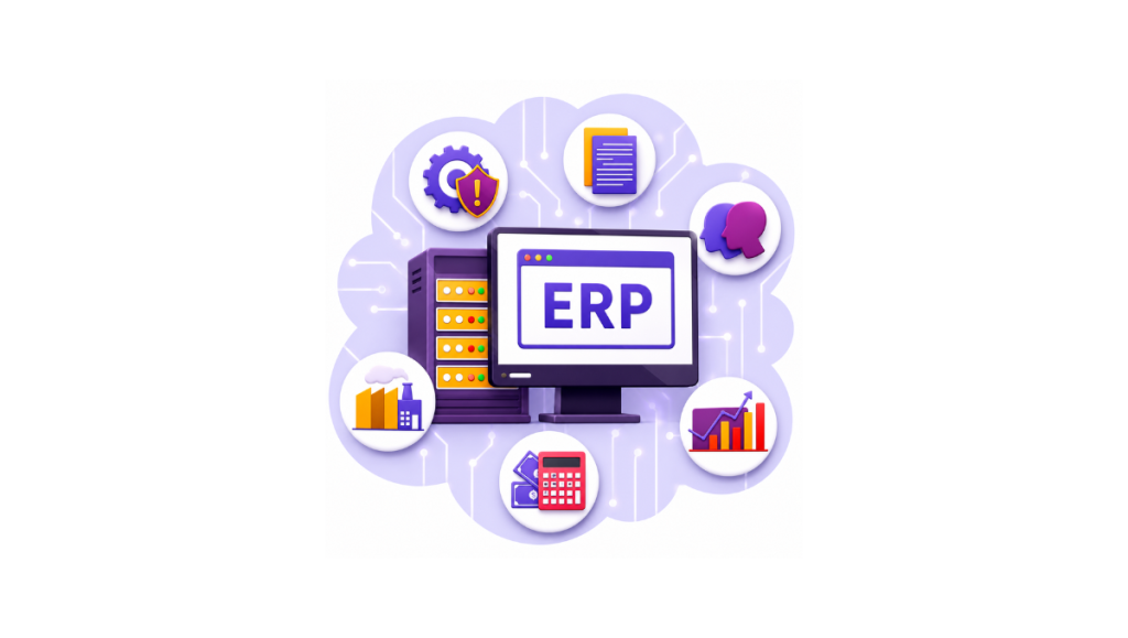
ERP Systems are in High Demand

ERP software is now an important element of any modern business. ERP combines finance, inventory, purchase management, sales, manufacturing, and human resource management into one system.

Thus, rather than using different programs, a company can control all its activities with just one software application. It increases efficiency, decreases duplication, and helps to get information in real time.

A lot of multinational enterprises apply ERP systems such as SAP or Oracle. Accountants who know how to use ERP are greatly appreciated since they are able to control financial processes and help other departments at the same time.

Automation is Improving Accuracy

Automation has significantly reduced manual accounting work. Tasks such as bank reconciliation, invoice processing, payroll calculations, expense approvals, and report generation can now be completed automatically using specialised software.

By automating routine work, accountants can dedicate more time to financial planning, auditing, and strategic analysis. Automation also minimises errors caused by manual data entry, resulting in more accurate financial records.

Learning automation tools has become essential for professionals who want to remain competitive in today’s technology-driven workplace.

Business Intelligence Tools are Becoming Essential

BI tools allow organisations to transform financial data into interactive dashboards and reports. Instead of analysing lengthy spreadsheet reports, management is able to comprehend how the business is performing using various charts and real-time dashboards.

The accountant plays an essential role in the creation of such reports because he/she knows more about financial data than any other person. Knowledge of software such as Power BI allows one to communicate information effectively and make decisions faster.

With organisations adopting data-driven approaches, BI skills have become a crucial aspect of an accountant’s skill set.

Cybersecurity Awareness is No Longer Optional

Financial data forms one of the most precious assets of an organisation. With accounting becoming more technologically advanced, it becomes imperative to secure this precious asset.

It becomes necessary for accountants to have knowledge regarding basic cybersecurity principles such as password creation, multi-factor authentication, phishing attacks, and confidentiality of financial data.

While it is the job of cybersecurity professionals to handle the security systems, it is equally important for accountants to ensure the confidentiality of financial data.

Blockchain is Creating New Opportunities

The accounting field has slowly been adopting the use of blockchain through offering secure and transparent records of transactions. The use of blockchain in offering permanent and tamper-proof transaction records makes it possible to offer improved audits and prevent any cases of fraud.

While the use of blockchain has not yet been fully adopted, having an idea about it may prepare the ground for future work.

The Importance of Continuous Learning

With each passing year, technology keeps developing further, and thus,, there is a need for accountants to have the skill of lifelong learning. Those who are able to continuously update themselves become more important in their work and grow better in their careers.

Being able to use different accounting programs, mastering advanced Excel skills, getting familiar with data analytics, and being updated about the developments in the field all make one successful in their career.

It is equally important for students to gain practical experience rather than only theoretical knowledge.

If you are planning to start your career, enrolling in job-oriented emerging technology courses in Bangalore can provide practical exposure to the latest accounting tools and industry practices. Such programs help bridge the gap between classroom learning and workplace expectations.

Similarly, choosing professional accounting training in Bangalore allows students and working professionals to develop practical skills that employers actively seek. Learning from experienced industry professionals also improves confidence during interviews and on the job.

Building the Best Accounting Career in 2026

Every year, technology moves ahead, which means that it is necessary for accountants to be able to learn throughout their lives. Those who manage to do this are becoming more and more valuable for their job and are becoming more successful in their careers.

Knowledge of various programs used in accounting, advanced skills in using Excel, being aware of what is going on in the field of data analytics, and other similar factors make one successful.

The same is valid for students who need to get practical experience rather than theoretical knowledge.

If your goal is to build the best accounting career, investing time in learning emerging technologies is one of the smartest decisions you can make. The accounting profession will continue to evolve, and those who adapt to change will enjoy long-term success.

Conclusion

The future of accounting lies in the hands of those accountants who possess not only the basics of accounting but also advanced technological know-how. The corporate world is embracing digitisation at a very fast pace to ensure efficiency and accuracy in its operations.

Learning accounting technologies is no longer an added advantage; it has become a necessity. Whether you are beginning your career or looking to advance professionally, embracing emerging technologies will help you stay competitive in the evolving job market. By continuously upgrading your skills and gaining practical experience, you can prepare yourself for exciting opportunities and become a future-ready accounting professional.

FAQs

1. Why should accountants acquire knowledge of new technologies?

New technologies assist accountants in automating their work, increasing precision, working with financial data effectively, and making better business decisions.

2. What is the most crucial technology for accountants in 2026?

Artificial Intelligence, Cloud Accounting, ERP Systems, Data Analytics, Business Intelligence Software, and Automation are some of the most crucial technologies for accountants in the modern world.

3. Is it better to use cloud accounting rather than traditional accounting software?

Yes, because cloud accounting enables real-time access to financial data, improves collaboration, provides backup solutions, and ensures that companies can operate from anywhere safely.

4. Should students of accounting learn data analytics?

Yes, because data analytics allows accountants to make sense out of the information about finances and spot trends.

5. How can I prepare for an accounting job with technologies?

Learn both fundamental accounting principles and modern accounting software, ERP Systems, cloud accounting, artificial intelligence, automation, and data analytics.

The accounting profession has experienced a tremendous change over the last decade. Previously, accounting practitioners were concerned mainly with the tasks of bookkeeping, accounting, taxation, and auditing. Although all these functions are still essential, today’s companies require accounting practitioners to provide more insights, which will be helpful for making decisions strategically.

Such changes have occurred due to the increased access to financial data and the development of analytical tools. Companies do not need accountants who just make records. They require accountants who can analyse financial data, make predictions, and help in making business decisions.

As a result, Data analysis in accounting has become one of the most valuable skills for accounting professionals. The ability to analyse financial information and turn it into actionable insights is redefining career opportunities and creating new paths for growth in the accounting industry.

The Evolution of Accounting in the Digital Age

Management of finances was always the core function of accounting. The amount of information produced by organisations now, however, is much greater than it has ever been.

Modern organisations employ several systems related to sales, stock control, customer relations management, payroll, and finance. A vast amount of information is produced daily. Merely recording the information is not enough anymore.

Modern accountants are expected to:

• Analyse business performance
• Identify financial risks
• Improve operational efficiency
• Support budgeting and forecasting
• Provide recommendations for growth

Technology has automated many routine accounting tasks. This has allowed accountants to focus more on interpretation and strategic planning rather than manual data entry.

Why Financial Data Analysis Matters?

Financial data tells the story of a business. Every transaction, expense, sale, and investment contributes to understanding how an organisation performs.

When analysed effectively, financial data can reveal:

• Revenue growth patterns
• Cost-saving opportunities
• Cash flow challenges
• Customer profitability
• Investment performance
• Future financial risks

Business leaders rely on these insights to make informed decisions. This is why the importance of analytics in accounting continues to grow across industries.

Instead of preparing reports that look at the past, accountants are increasingly helping organisations predict future outcomes and develop proactive strategies.

The Shift from Traditional Accountant to Strategic Advisor

The role of an accountant is changing at an incredibly fast pace. The modern finance experts are not record keepers but advisors. 

Take a situation where there is a decline in the profits of the company, and the management requires an understanding of why it has occurred. A financially savvy accountant will be able to analyse the sales figures, operating expenses, cost of inventories, and consumer behaviour to determine what causes the profit decline.

Likewise, during the expansion process, an accountant can use financial performance from the past and market trends to predict future income and expenses.

Technologies Driving Financial Data Analysis

Several technologies have contributed to the growing demand for analytical skills in accounting.

Business Intelligence Tools

Platforms such as Power BI and Tableau help accountants visualise financial information through interactive dashboards and reports. These tools make complex data easier to understand and communicate.

Cloud Accounting Systems

Cloud-based accounting software provides real-time access to financial information. This allows accountants to monitor performance continuously and respond quickly to changes.

Artificial Intelligence and Automation

AI-powered systems can process large volumes of financial data, identify patterns, and generate forecasts. Accountants can use these insights to make more accurate recommendations.

Advanced Spreadsheet Analytics

Modern Excel features, including Power Query, Pivot Tables, and Power Pivot, enable professionals to perform sophisticated financial analysis efficiently.

Together, these technologies are transforming the accounting profession and increasing the demand for data-driven decision-making.

How do Data Analysis Skills Improve Career Opportunities?

Employers today seek accounting professionals who can go beyond traditional accounting functions.

Candidates with analytical skills often enjoy advantages such as:

Better Job Prospects

Organisations increasingly prefer accountants who understand both finance and analytics. These professionals can contribute more effectively to business strategy and performance management.

Higher Salaries

Specialised skills often lead to higher compensation. Professionals who can analyse data, create dashboards, and generate business insights are highly valued in the job market.

Expanded Career Paths

Analytical expertise opens opportunities in various roles, including:

• Financial Analyst
• Business Analyst
• Management Accountant
• Financial Planning and Analysis (FP&A) Professional
• Data Analyst
• Risk Analyst
• Finance Manager

Many accountants are successfully transitioning into broader business and analytical roles because of their financial expertise combined with data skills.

Real-World Applications of Financial Data Analysis

Financial data analysis is no longer limited to large corporations. Businesses of all sizes use analytics to improve decision-making.

Budget Planning

Organisations analyse historical spending patterns to create realistic budgets and control costs more effectively.

Cash Flow Management

By examining cash inflows and outflows, businesses can predict potential shortages and maintain healthy liquidity.

Profitability Analysis

Companies use financial data to determine which products, services, or customers generate the highest profits.

Fraud Detection

Advanced analytics can identify unusual transactions and patterns that may indicate fraud or financial irregularities.

Investment Decisions

Financial analysis helps businesses evaluate investment opportunities and estimate potential returns.

These applications demonstrate how analytical skills directly contribute to business success.

Skills Modern Accountants Need

To remain competitive in today’s market, accountants must develop a combination of technical and analytical skills.

Important skills include:

Financial Reporting Knowledge

A strong understanding of accounting principles remains essential.

Data Visualization

]The ability to present complex financial information clearly helps stakeholders make informed decisions.

Statistical Analysis

Basic statistical knowledge supports trend analysis and forecasting.

Business Intelligence Tools

Proficiency in tools such as Power BI and Tableau is increasingly valuable.

Critical Thinking

Accountants must interpret data, identify patterns, and recommend practical solutions.

Insights are only useful when communicated effectively to management and decision-makers.

Professionals who combine these skills can significantly enhance their career prospects.

The Growing Demand for Data-Driven Accountants

Modern business enterprises have to face extremely competitive situations. Accountants have all the necessary skills and expertise to supply decision makers with timely and accurate information.

It is a well-known fact that industry trends prove the rising value of the specialists who can establish a connection between finance and technology.

Organisations want professionals who can answer critical questions such as:

• Why are profits increasing or decreasing?
• Which products generate the highest margins?
• What financial risks could affect future growth?
• How can operational costs be reduced?

Answering these questions requires strong analytical capabilities.

Learning Financial Analytics for Career Growth

The good news is that analytical skills can be learned through structured training and practical experience.

Many accounting professionals are enhancing their expertise through specialised programs that focus on:

• Data visualization
• Financial analytics
• Business intelligence tools
• Dashboard creation
• Data interpretation
• Forecasting techniques

Enrolling in a Data analytics course can help aspiring accountants gain hands-on experience with industry-standard tools and analytical methodologies.

Professionals seeking career advancement often choose the finance courses in bangalore that combines finance concepts with practical analytical applications. Such programs help bridge the gap between traditional accounting knowledge and modern business requirements.

The Future of Accounting Careers

The future of accounting is closely tied to data and technology. While automation will continue to handle routine tasks, the need for human judgment, interpretation, and strategic thinking will remain strong.

Accountants who embrace analytics will be better positioned to

• Deliver business insights
• Support organizational growth
• Improve financial performance
• Advance into leadership roles

Rather than replacing accountants, technology is enhancing their value by enabling them to focus on higher-level responsibilities.

As businesses become increasingly data-driven, professionals who master Data analysis in accounting will enjoy greater career opportunities and long-term success.

Conclusion

Data analysis is changing the accounting profession in a profound way. Nowadays, accountants are not just supposed to keep books and produce reports. They have to analyse financial information, extract knowledge from it and be involved in making strategic decisions based on the findings.

The emergence of analytical tools and applications gives great chances to those accountants who are ready to acquire new skills and competencies. With this help, they will be able to enhance their career perspectives and become more valuable to organisations.

It goes without saying that in the future there will be demand for such professionals who are capable of turning financial data into useful business information. For an accountant, it will be a great opportunity, rather than a threat.

FAQs

1. What is the definition of Financial data analysis in accounting?

Financial data analysis is defined as the process of analysing financial data to establish trends, performance, forecasting, and help in business decisions.

2. What is the Importance of data analysis in the career of an accountant?

Data analysis skills allow accountants to go beyond conventional bookkeeping to provide strategies that make the business more profitable.

3. Which are the softwares used for financial data analysis?

Some of the software used in financial data analysis include Excel, Power BI, Tableau, cloud-based accounting software, and other business intelligence tools.

4. Can accountants be data analysts?

Yes. This is because accountants are knowledgeable in finance and would find it easy to acquire analysis skills.

5. How do I learn financial data analysis?

It is possible to learn financial data analysis from certifications, online courses, workshops, and a Data analytics course in Bangalore by using business data.